More SciPy#
import numpy as np
import matplotlib.pyplot as plt
Fitting#
Fitting is used to match a model to experimental data. E.g. we have N points of \((x_i, y_i)\) with associated errors, \(\sigma_i\), and we want to find a simple function that best represents the data.
Usually this means that we will need to define a metric, often called the residual, for how well our function matches the data, and then minimize this residual. Least-squares fitting is a popular formulation.
We want to fit our data to a function \(Y(x, \{a_j\})\), where \(a_j\) are model parameters we can adjust. We want to find the optimal \(a_j\) to minimize the distance of \(Y\) from our data, measured parallel to the \(y\)-axis:
Least-squares minimizes the distance between the data points and the model line parallel to the \(y\)-axis. We write this as \(\chi^2\):
from scipy import optimize
general linear least squares#
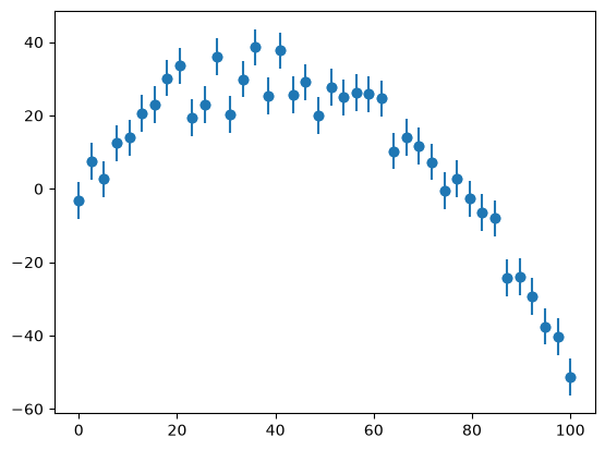
First we’ll make some experimental data (a quadratic with random fashion). We use the standard_normal function to provide Gaussian normalized errors.
def y_experiment2(a1, a2, a3, sigma, x):
    """ return the experimental data in a quadratic + random fashion,
        with a1, a2, a3 the coefficients of the quadratic and sigma is
        the error.  This will be poorly matched to a linear fit for
        a3 != 0 """

    N = len(x)

    # standard_normal gives samples from the "standard normal" distribution
    rng = np.random.default_rng()
    r = rng.standard_normal(N)

    y = a1 + a2*x + a3*x*x + sigma*r

    return y
N = 40
sigma = 5.0*np.ones(N)

x = np.linspace(0, 100.0, N)
y = y_experiment2(2.0, 1.50, -0.02, sigma, x)
fig, ax = plt.subplots()
ax.scatter(x,y)
ax.errorbar(x, y, yerr=sigma, fmt="o")
<ErrorbarContainer object of 3 artists>
Note
“linear” in general linear least squares means that the fit parameters enter into the fitting function linearly, the function itself can be nonlinear in \(x\).
We’ll use the leastsq() function to minimize the square of the residual.
First our function to compute the residual.
def resid(avec, x, y, sigma):
    """ the residual function -- this is what will be minimized by the
        scipy.optimize.leastsq() routine.  avec is the parameters we
        are optimizing -- they are packed in here, so we unpack to
        begin.  (x, y) are the data points

        scipy.optimize.leastsq() minimizes:

           x = arg min(sum(func(y)**2,axis=0))
                    y

        so this should just be the distance from a point to the curve,
        and it will square it and sum over the points
        """

    a0, a1, a2 = avec

    return (y - (a0 + a1*x + a2*x**2))/sigma
# initial guesses
a0, a1, a2 = 1, 1, 1

afit, flag = optimize.leastsq(resid, [a0, a1, a2], args=(x, y, sigma))

print(afit)
[ 0.77686434 1.59026776 -0.02084646]
ax.plot(x, afit[0] + afit[1]*x + afit[2]*x*x )
fig
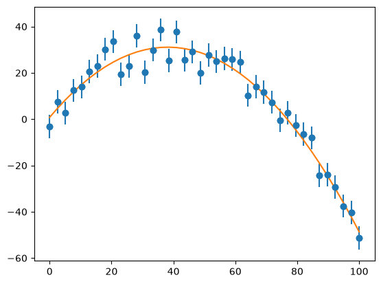
We see that we represent the data quite well.
We can compute the reduced \(\chi^2\)
chisq = sum(np.power(resid(afit, x, y, sigma),2))
normalization = len(x)-len(afit)
print(chisq/normalization)
0.9409896163330335
In general a (reduced) \(\chi^2 < 1\) indicates a good fit.
a nonlinear example#
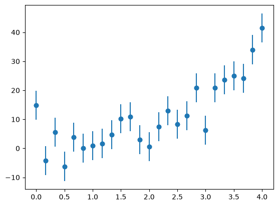
The same interface works with nonlinear data.
We’ll create a new set of experimental data—an exponential
a0 = 2.5
a1 = 2./3.
sigma = 5.0

a0_orig, a1_orig = a0, a1

rng = np.random.default_rng()

x = np.linspace(0.0, 4.0, 25)
y = a0*np.exp(a1*x) + sigma * rng.standard_normal(len(x))
fig, ax = plt.subplots()
ax.scatter(x,y)
ax.errorbar(x, y, yerr=sigma, fmt="o", label="_nolegend_")
<ErrorbarContainer object of 3 artists>
our function to minimize
def resid(avec, x, y):

    a0, a1 = avec

    # note: if we wanted to deal with error bars, we would weight each
    # residual accordingly
    return y - a0*np.exp(a1*x)
a0, a1 = 1, 1
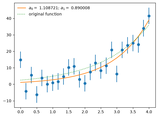
afit, flag = optimize.leastsq(resid, [a0, a1], args=(x, y))
print(flag)
print(afit)
1
[1.10872096 0.89000762]
ax.plot(x, afit[0]*np.exp(afit[1]*x),
           label=r"$a_0 = $ %f; $a_1 = $ %f" % (afit[0], afit[1]))
ax.plot(x, a0_orig*np.exp(a1_orig*x), ":", label="original function")
ax.legend(numpoints=1, frameon=False)
fig
Note
What about uncertainties in both \(x\) and \(y\)? SciPy has an orthogonal distance regression implementation based on ODRPACK for this.
FFTs#
Fourier transforms convert a physical-space (or time series) representation of a function into frequency space. This provides an equivalent representation of the data with a new view.
The FFT and its inverse in NumPy use:
Both NumPy and SciPy have FFT routines that are similar. However, the NumPy version returns the data in a more convenient form.
Tip
It’s always best to start with something you understand—let’s do a simple sine wave. Since our function is real, we can use the rfft routines in NumPy—the understand that we are working with real data and they don’t return the negative frequency components.
Important
FFTs assume that you are periodic. If you include both endpoints of the domain in the points that comprise your sample then you will not match this assumption. Here we use endpoint=False with linspace()
Note
For real-valued data, we’ll use np.fft.rfft(), which will return N/2 complex values given N real samples.
To get the frequencies, we can use np.fft.rfftfreq(), which will return dimensionless frequencies of the form
\(0, 1/N, 2/N, 3/N, ...\). We know that the shortest lowest frequency corresponds to a single wavelength in the domain, so physically, \(1/N\) corresponds to a frequency \(1/L\), where \(L\) is the domain size. This means that
we can convert the frequencies by dividing by \(\Delta x = L/N\). This scaling is accomplished by passing the
d parameter to rfftfreq.
To make our life easier, we’ll define a function that plots all the stages of the FFT process
def plot_FFT(xx, f):

    npts = len(xx)
    dx = xx[1] - xx[0]

    # Forward transform: f(x) -> F(k)
    fk = np.fft.rfft(f)

    # Normalization -- the '2' here comes from the fact that we are
    # neglecting the negative portion of the frequency space, since
    # the FFT of a real function contains redundant information, so
    # we are only dealing with 1/2 of the frequency space.
    #
    # technically, we should only scale the 0 bin by N, since k=0 is
    # not duplicated -- we won't worry about that for these plots
    norm = 2.0 / npts

    fk = fk * norm

    # rfftfreq returns the frequencies as 0, 1/N, 2/N, 3/N, ...
    kfreq = np.fft.rfftfreq(npts, d=dx)

    # Inverse transform: F(k) -> f(x) -- without the normalization
    fkinv = np.fft.irfft(fk/norm)

    # plots
    fig, ax = plt.subplots(nrows=4, ncols=1)

    ax[0].plot(xx, f)
    ax[0].set_xlabel("x")
    ax[0].set_ylabel("f(x)")

    ax[1].plot(kfreq, fk.real, label=r"Re($\mathcal{F}$)")
    ax[1].plot(kfreq, fk.imag, ls=":", label=r"Im($\mathcal{F}$)")
    ax[1].set_xlabel(r"$\nu_k$")
    ax[1].set_ylabel("F(k)")

    ax[1].legend(fontsize="small", frameon=False)

    ax[2].plot(kfreq, np.abs(fk))
    ax[2].set_xlabel(r"$\nu_k$")
    ax[2].set_ylabel(r"|F(k)|")

    ax[3].plot(xx, fkinv.real)
    ax[3].set_xlabel(r"$\nu_k$")
    ax[3].set_ylabel(r"inverse F(k)")

    fig.set_size_inches(10,8)
    fig.tight_layout()
Now we’ll test it on \(f(x) = \sin(2\pi \nu_0 x)\), where \(\nu_0\) is a frequency we set.
def single_freq_sine(npts):

    # a pure sine with no phase shift will result in pure imaginary
    # signal
    f_0 = 0.2

    xmax = 10.0/f_0

    xx = np.linspace(0.0, xmax, npts, endpoint=False)

    f = np.sin(2.0*np.pi*f_0*xx)

    return xx, f
npts = 128
xx, f = single_freq_sine(npts)
plot_FFT(xx, f)
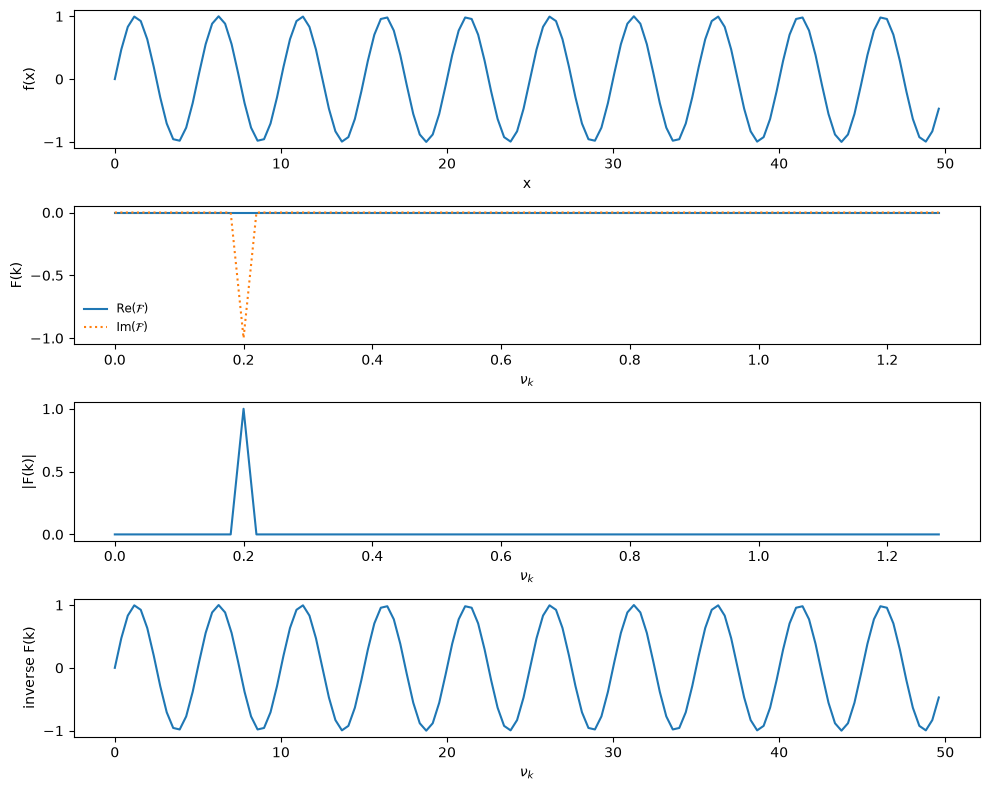
Notice that all of the power is at our single frequency, and it is all in the imaginary components, which is expected since \(e^{ix} = \cos(x) + i\sin(x)\)
Next, we can try \(f(x) = \cos(2\pi\nu_0 x)\), and we know that a cosine is just a sine shifted in phase by \(\pi/2\).
def single_freq_cosine(npts):

    # a pure cosine with no phase shift will result in pure real
    # signal
    f_0 = 0.2

    xmax = 10.0/f_0

    xx = np.linspace(0.0, xmax, npts, endpoint=False)

    f = np.cos(2.0*np.pi*f_0*xx)

    return xx, f
xx, f = single_freq_cosine(npts)
plot_FFT(xx, f)
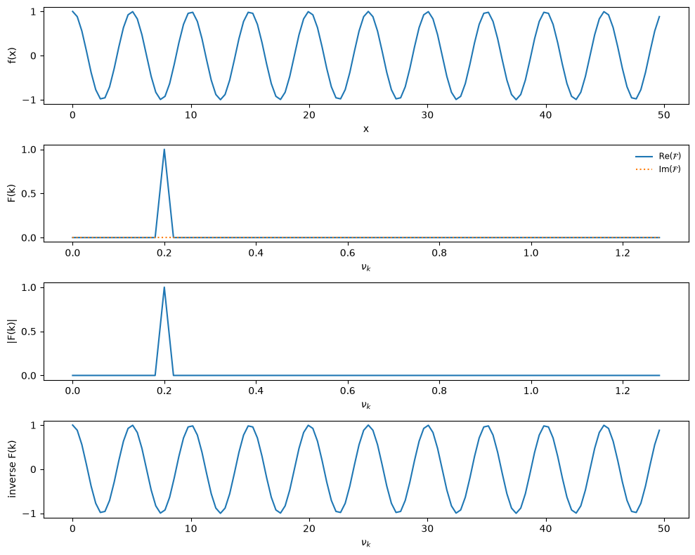
Now, as expected, all of the power is in the real component.
Now let’s look at a sine with a \(\pi/4\) phase shift
def single_freq_sine_plus_shift(npts):

    # a pure sine with no phase shift will result in pure imaginary
    # signal
    f_0 = 0.2

    xmax = 10.0/f_0

    xx = np.linspace(0.0, xmax, npts, endpoint=False)

    f = np.sin(2.0*np.pi*f_0*xx + np.pi/4)

    return xx, f
xx, f = single_freq_sine_plus_shift(npts)
plot_FFT(xx, f)
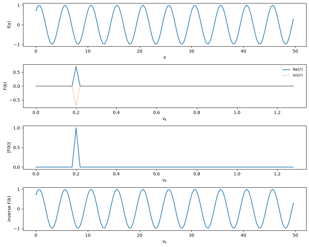
No surprise—the power is now equally in the real and imaginary parts.
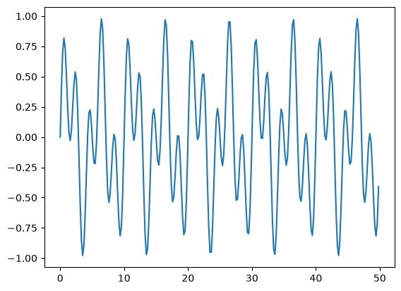
A frequency filter#
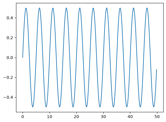
we’ll setup a simple two-frequency sine wave and filter a component
def two_freq_sine(npts):

    # a pure sine with no phase shift will result in pure imaginary
    # signal
    f_0 = 0.2
    f_1 = 0.5

    xmax = 10.0/f_0

    # we call with endpoint=False -- if we include the endpoint, then for
    # a periodic function, the first and last point are identical -- this
    # shows up as a signal in the FFT.
    xx = np.linspace(0.0, xmax, npts, endpoint=False)

    f = 0.5*(np.sin(2.0*np.pi*f_0*xx) + np.sin(2.0*np.pi*f_1*xx))

    return xx, f
npts = 256

xx, f = two_freq_sine(npts)

fig, ax = plt.subplots()
ax.plot(xx, f)
[<matplotlib.lines.Line2D at 0x7fdb91b623c0>]
we’ll take the transform: \(f(x) \rightarrow F(k)\)
# normalization factor: the 2 here comes from the fact that we neglect
# the negative portion of frequency space because our input function
# is real
norm = 2.0/npts
fk = norm*np.fft.rfft(f)

ofk_r = fk.real.copy()
ofk_i = fk.imag.copy()

# get the frequencies
k = np.fft.rfftfreq(len(xx))

# since we don't include the endpoint in xx, to normalize things, we need
# max(xx) + dx to get the true length of the domain
#
# This makes the frequencies essentially multiples of 1/dx
kfreq = k*npts/(max(xx) + xx[1])
fig, ax = plt.subplots()
ax.plot(kfreq, fk.real, label="real")
ax.plot(kfreq, fk.imag, ":", label="imaginary")
ax.legend(frameon=False)
<matplotlib.legend.Legend at 0x7fdb91bb3620>
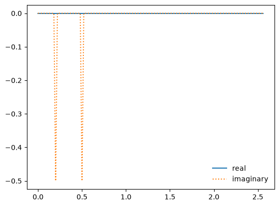
Now we can filter out the higher frequencies—this is done in Fourier space.
fk[kfreq > 0.4] = 0.0
Finally, transform back.
# Inverse transform: F(k) -> f(x)
fkinv = np.fft.irfft(fk/norm)
fig, ax = plt.subplots()
ax.plot(xx, fkinv.real)
[<matplotlib.lines.Line2D at 0x7fdb91a64830>]
Linear Algebra#
general manipulations of matrices#
You can use regular NumPy arrays or you can use a special matrix class that offers some short cuts.
Tip
Since the introduction of the matrix multiplication operator, @, using the numpy matrix class is no longer recommended.
Let’s create a simply 2x2 matrix, \({\bf A}\)
a = np.array([[1.0, 2.0],
              [3.0, 4.0]])
print(a)
print(a.transpose())
print(a.T)
[[1. 2.]
 [3. 4.]]
[[1. 3.]
 [2. 4.]]
[[1. 3.]
 [2. 4.]]
We can solve for the inverse
ainv = np.linalg.inv(a)
print(ainv)
[[-2.   1. ]
 [ 1.5 -0.5]]
And multiply \({\bf A}\) by its inverse, \({\bf A}^{-1}\)
a @ ainv
array([[1.0000000e+00, 0.0000000e+00],
       [8.8817842e-16, 1.0000000e+00]])
the eye() function will generate an identity matrix (as will the identity())
print(np.eye(2))
print(np.identity(2))
[[1. 0.]
 [0. 1.]]
[[1. 0.]
 [0. 1.]]
Linear systems#
we can solve \({\bf A}{\bf x} = {\bf b}\) easily.
Note
Linear system solvers don’t usually compute the inverse first and then multiply by it. It is much cheaper to solve the system directly (e.g., via Gaussian elimination) than to first compute the inverse.
b = np.array([5, 7])
x = np.linalg.solve(a, b)
print(x)
[-3. 4.]
tridiagonal matrix solve#
Here we’ll solve the Poisson problem:
with \(g(x) = \sin(x)\), and the domain \(x \in [0, 2\pi]\), with boundary conditions \(f(0) = f(2\pi) = 0\).
The solution is simply \(f(x) = -\sin(x)\).
We’ll use a grid of \(N\) points with \(x_0\) on the left boundary and \(x_{N-1}\) on the right boundary.
We difference our equation as:
We keep the boundary points fixed, so we only need to solve for the \(N-2\) interior points. Near the boundaries, our difference is:
and
We can write the system of equations for solving for the \(N-2\) interior points as:
Then we just solve \({\bf A}{\bf x} = {\bf b}\)
Note
SciPy has banded solvers that work with banded matrices like we have above. They will be much more efficient than using a solver based on a dense matrix
import scipy.linalg as linalg

# our grid -- including endpoints
N = 100
x = np.linspace(0.0, 2.0*np.pi, N, endpoint=True)
dx = x[1] - x[0]

# our source
g = np.sin(x)

# our matrix will be tridiagonal, with [1, -2, 1] on the diagonals
# we only solve for the N-2 interior points

# diagonal
d = -2 * np.ones(N-2)

# upper -- note that the upper diagonal has 1 less element than the
# main diagonal.  The SciPy banded solver wants the matrix in the
# form:
#
# *    a01  a12  a23  a34  a45    <- upper diagonal
# a00  a11  a22  a33  a44  a55    <- diagonal
# a10  a21  a32  a43  a54   *     <- lower diagonal
#

u = np.ones(N-2)
u[0] = 0.0

# lower
l = np.ones(N-2)
l[N-3] = 0.0

# put the upper, diagonal, and lower parts together as a banded matrix
A = np.matrix([u, d, l])

# solve A sol = dx**2 g for the inner N-2 points
sol = linalg.solve_banded((1,1), A, dx**2*g[1:N-1])
Let’s plot the solution
fig, ax = plt.subplots()
ax.plot(x[1:N-1], sol)
[<matplotlib.lines.Line2D at 0x7fdb91ad4d70>]
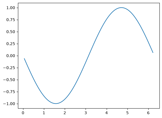
This looks like \(-\sin(x)\), as expected.