Machine Learning Introduction#
Neural networks#
When we talk about machine learning, we usually mean an artifical neural network. A neural network mimics the action of neurons in your brain.
Basic idea:
Create a nonlinear fitting routine with free parameters
Train the network on data with known inputs and outputs to set the parameters
Use the trained network on new data to predict the outcome
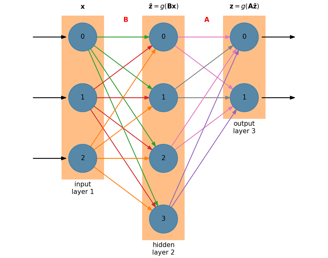
We can think of a neural network as a map that takes a set of n parameters and returns a set of m parameters, \(\mathbb{R}^n \rightarrow \mathbb{R}^m\) and we can express this as:
where \({\bf x} \in \mathbb{R}^n\) are the inputs, \({\bf z} \in \mathbb{R}^m\) are the outputs, and \({\bf A}\) is an \(m \times n\) matrix.
Our goal is to determine the matrix elements of \({\bf A}\).
Some nomeclature#
We can visualize a neural network as:
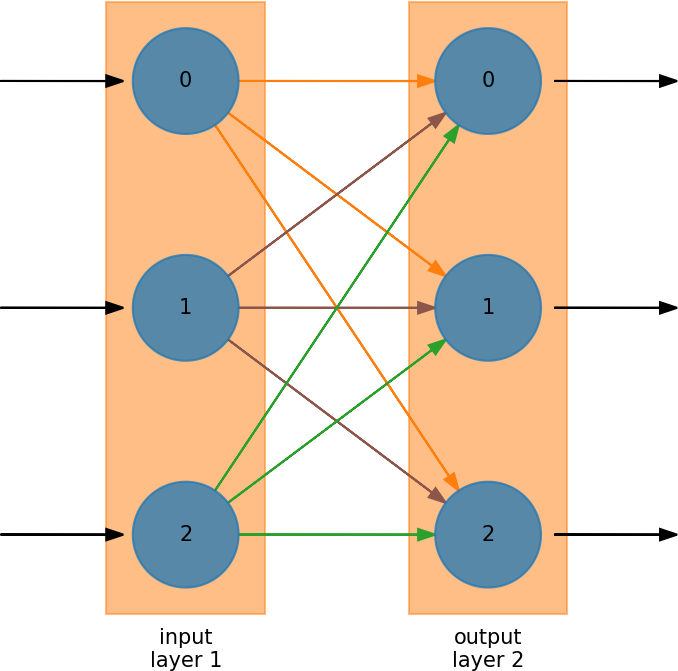
Neural networks are divided into layers
There is always an input layer—it doesn’t do any processing
There is always an output layer
Within a layer there are neurons or nodes.
For input, there will be one node for each input variable.
Every node in the first layer connects to every node in the next layer
The weight associated with the connection can vary—these are the matrix elements.
In this example, the processing is done in layer 2 (the output)
When you train the neural network, you are adjusting the weights connecting to the nodes
Some connections might have zero weight
This mimics nature—a single neuron can connect to several (or lots) of other neurons.
Universal approximation theorem and non-linearity#
A neural network can be designed to approximate any function, \(f(x)\). For this to work, there must be a source of non-linearity in the network. This is applied on a layer. This is a result of the universal approximation theorem.
We call this an activation function and it has the form:
Then our neural network has the form: \({\bf z} = g({\bf A x})\)
We want to choose a \(g(x)\) that is differentiable. A common choice is the sigmoid function:
import numpy as np
import matplotlib.pyplot as plt
def sigmoid(p):
    return 1 / (1 + np.exp(-p))
p = np.linspace(-10, 10, 200)

fig, ax = plt.subplots()

ax.plot(p, sigmoid(p))
[<matplotlib.lines.Line2D at 0x7f3cb11dccd0>]
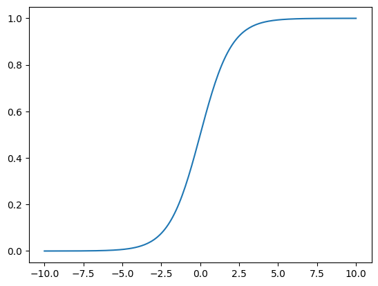
Notice that the sigmoid scales all output to be in \(z_i \in (0, 1)\)
This means that we need to ensure that our training set set is likewise mapped to \((0, 1)\), and if not, we need to transform it.
Basic algorithm#
Training
We have \(T\) pairs \((x^k, y^k)\) for \(k = 1, \ldots, T\)
We require that \(g({\bf A x}^k) = {\bf y}^k\) for all \(k\)
Recall that \(g(p)\) is a scalar function that works element-by-element:
\[z_i = g([{\bf A x}]_i) = g \left ( \sum_j A_{ij} x_j \right )\]Find the elements of \({\bf A}\)
This is a minimization problem, where we are minimizing:
\[f(A_{ij}) = \| g({\bf A x}^k) - {\bf y}^k \|^2\]We call this function the cost function.
A common minimization technique is gradient descent.
Some caveats:
When you minimize with one set of training data, there is no guarantee that your are still minimimzed with respect to the others. We do multiple epochs or passes through the training data to fix this.
We often don’t apply the full correction from gradient descent, but instead scale it by some \(\eta < 1\) called the learning rate.
Using the network
With the trained \({\bf A}\), we can now use the network on data we haven’t seen before